R4DS讀到現在,覺得這真是本很棒的入門書,tidyverse裡面的package一脈相承的設計哲學讓data manipulation可以系統化的學習,而非只是死背一卡車的函數。尤其dplyr,函數操作濃濃的SQL味道,很容易上手,讀到這裡終於有信心用R做前處理,而不是看完整本書覺得腦子裡只有碎片化的函數飛來飛去……
第五章最末兩小節的練習題特別多且應用性強,故獨立一篇記錄之。
Exercise 5.6.2
Come up with another approach that will give you the same output as not_cancelled %>% count(dest) and not_cancelled %>% count(tailnum, wt = distance) (without using count())
#not_cancelled %>% count(dest)

#not_cancelled %>%
#  group_by(dest) %>%
#  summarise(n = n())

#not_cancelled %>%
#  group_by(dest) %>%
#  summarise(n = length(dest))
# using summarise() to create one or more scalar variables
# summarizing the variables of an existing tbl
# summarise(), to reduce multiple values down to a single value

# count() is effectively a short-cut for group_by() followed by # tally()
#not_cancelled %>%
#  group_by(dest) %>%
#  tally()

#> # A tibble: 104 x 2
#>   dest      n
#>   <chr> <int>
#> 1 ABQ     254
#> 2 ACK     264
#> 3 ALB     418
#> 4 ANC       8
#> 5 ATL   16837
#> 6 AUS    2411
#> # … with 98 more rows
# not_cancelled %>% count(tailnum, wt = distance)

#not_cancelled %>%
#  group_by(tailnum) %>%
#  summarise(n = sum(distance))

# we can also use the combination group_by() and tally().
# any arguments to tally() are summed.
not_cancelled %>%
  group_by(tailnum) %>%
  tally(distance)

#> # A tibble: 4,037 x 2
#>   tailnum      n
#>   <chr>    <dbl>
#> 1 D942DN    3418
#> 2 N0EGMQ  239143
#> 3 N10156  109664
#> 4 N102UW   25722
#> 5 N103US   24619
#> 6 N104UW   24616
#> # … with 4,031 more rows
Exercise 5.6.3
Our definition of cancelled flights (is.na(dep_delay) | is.na(arr_delay)) is slightly suboptimal. Why? Which is the most important column?
飛機起飛並不代表抵達,飛行過程可能發生意外或是折返回起飛機場,所以 arr_delay應該才是我們需要研究的目標column。
Exercise 5.6.4 *****
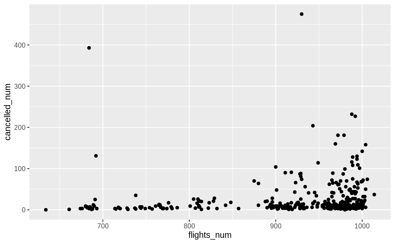
Look at the number of cancelled flights per day. Is there a pattern? Is the proportion of cancelled flights related to the average delay?
cancelled_per_day <-
  flights %>%
  mutate(cancelled = (is.na(arr_delay) | is.na(dep_delay))) %>%
# add a column "cancelled" , which show TRUE or FALSE
  group_by(year, month, day) %>%
  summarise(
    cancelled_num = sum(cancelled),
    flights_num = n(),
  )

# Plotting flights_num against cancelled_num
ggplot(cancelled_per_day) +
  geom_point(aes(x = flights_num, y = cancelled_num))

# with regression line
#  ggplot(cancelled_per_day, aes(x = flights_num, y = #cancelled_num)) +
#    geom_point() +
#    geom_smooth(method = "lm")
# 自己覺得畫出迴歸線後,發現 變數之間的關係不是很明顯

# whether there is a relationship between the proportion of
# flights cancelled and the average departure delay

cancelled_and_delays <-
  flights %>%
  mutate(cancelled = (is.na(arr_delay) | is.na(dep_delay))) %>%
  group_by(year, month, day) %>%
  summarise(
    cancelled_prop = mean(cancelled),
    avg_dep_delay = mean(dep_delay, na.rm = TRUE),
                                 # remove NA
    avg_arr_delay = mean(arr_delay, na.rm = TRUE)
  ) %>%
  ungroup()

  ggplot(cancelled_and_delays, aes(x = avg_dep_delay, y = cancelled_prop)) +
    geom_point() +
    geom_smooth(method = lm)

  ggplot(cancelled_and_delays, aes(x = avg_arr_delay, y = cancelled_prop)) +
    geom_point() +
    geom_smooth(method = lm)

Exercise 5.6.5
Which carrier has the worst delays?
Challenge: can you disentangle the effects of bad airports vs. bad carriers? Why/why not? (Hint: think about flights %>% group_by(carrier, dest) %>% summarise(n()))
flights %>%
  group_by(carrier) %>%
  summarise(arr_delay = mean(arr_delay, na.rm = TRUE)) %>%
  arrange(desc(arr_delay))
#> # A tibble: 16 x 2
#>   carrier arr_delay
#>   <chr>       <dbl>
#> 1 F9           21.9
#> 2 FL           20.1
#> 3 EV           15.8
#> 4 YV           15.6
#> 5 OO           11.9
#> 6 MQ           10.8
#> # … with 10 more rows


filter(airlines, carrier == "F9")
#> # A tibble: 1 x 2
#>   carrier name
#>   <chr>   <chr>
#> 1 F9      Frontier Airlines Inc.
Exercise 5.7.2
Which plane (tailnum) has the worst on-time record?The question does not define a way to measure on-time record, so I will consider two metrics:
1. proportion of flights not delayed or cancelled, and
2. mean arrival delay.
# 1.
on_time_prop_final <- flights %>%
  filter(!is.na(tailnum)) %>%
  mutate(on_time = (arr_delay <= 0)) %>%
  group_by(tailnum) %>%
  summarise(n = n(), on_time_prop = mean(on_time, na.rm = TRUE)) %>%
  arrange(on_time_prop)

# 2. mean arrival delay.
mean_arr_delay <- flights %>%
  filter(!is.na(tailnum)) %>%
  group_by(tailnum) %>%
  summarise(n = n(), avg_arr_delay = mean(arr_delay, na.rm = TRUE)) %>%
  arrange(desc(avg_arr_delay))

Exercise 5.7.3
What time of day should you fly if you want to avoid delays as much as possible?
best_hour <- flights %>%
  group_by(hour) %>%
  summarise(avg_arr_delay = mean(arr_delay, na.rm = TRUE),
            avg_dep_delay = mean(dep_delay, na.rm = TRUE)) %>%
  arrange(avg_arr_delay, avg_arr_delay)
Exercise 5.7.4
For each destination, compute the total minutes of delay. For each flight, compute the proportion of the total delay for its destination.
dest_delay_total <- flights %>%
  filter(arr_delay > 0) %>%
  group_by(dest) %>%
  mutate(
    arr_delay_total = sum(arr_delay),
    # using sum()
    arr_delay_prop = arr_delay / arr_delay_total
  ) %>%
  select(dest, arr_delay_total, arr_delay_prop)

Exercise 5.7.5 *****
Delays are typically temporally correlated: even once the problem that caused the initial delay has been resolved, later flights are delayed to allow earlier flights to leave. Using lag() explore how the delay of a flight is related to the delay of the immediately preceding flight.
lead-lag {dplyr} R Documentation
Description
Find the “next" or “previous" values in a vector. Useful for comparing values ahead of or behind the current values.
lag():這一筆與下一筆觀察值的差,等於下筆觀察值減這一筆觀察值。
lead():這一筆與前一筆觀察值的差,等於這一筆觀察值減前一筆觀察值。
Step 1.
Calculates the departure delay of the preceding flight from the same airport.
lagged_delays <- flights %>%
  arrange(origin, month, day, dep_time) %>%
  group_by(origin) %>%
  mutate(dep_delay_lag = lag(dep_delay)) %>%
  filter(!is.na(dep_delay), !is.na(dep_delay_lag))
Step 2.
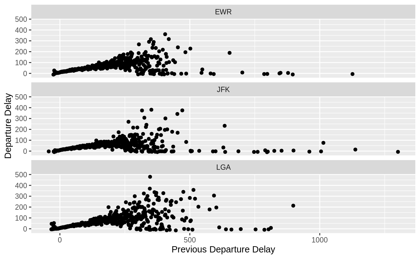
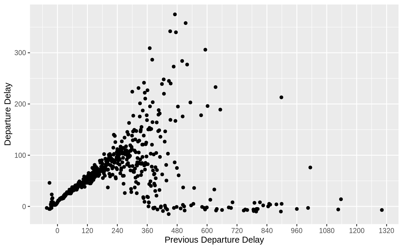
Plots the relationship between the mean delay of a flight for all values of the previous flight.
“Previous Departure Delay" against “Departure Delay"
lagged_delays %>%
  group_by(dep_delay_lag) %>%
  summarise(dep_delay_mean = mean(dep_delay)) %>%
  ggplot(aes(y = dep_delay_mean, x = dep_delay_lag)) +
  geom_point() +

# change distance between breaks for continuous x-axis ---
  scale_x_continuous(breaks = seq(0, 1500, by = 120)) +

  labs(y = "Departure Delay", x = "Previous Departure Delay")

“Previous Departure Delay" 與 “Departure Delay"之間的關係,在個別機場上或是 overall(所有機場的數據)的效果相似。
lagged_delays %>%
  group_by(origin, dep_delay_lag) %>%
  summarise(dep_delay_mean = mean(dep_delay)) %>%
  ggplot(aes(y = dep_delay_mean, x = dep_delay_lag)) +
  geom_point() +
  # facet_wrap() 分割子圖之參數設定
  facet_wrap(~origin, ncol = 1) +
  labs(y = "Departure Delay", x = "Previous Departure Delay")
Exercise 5.7.6 *****
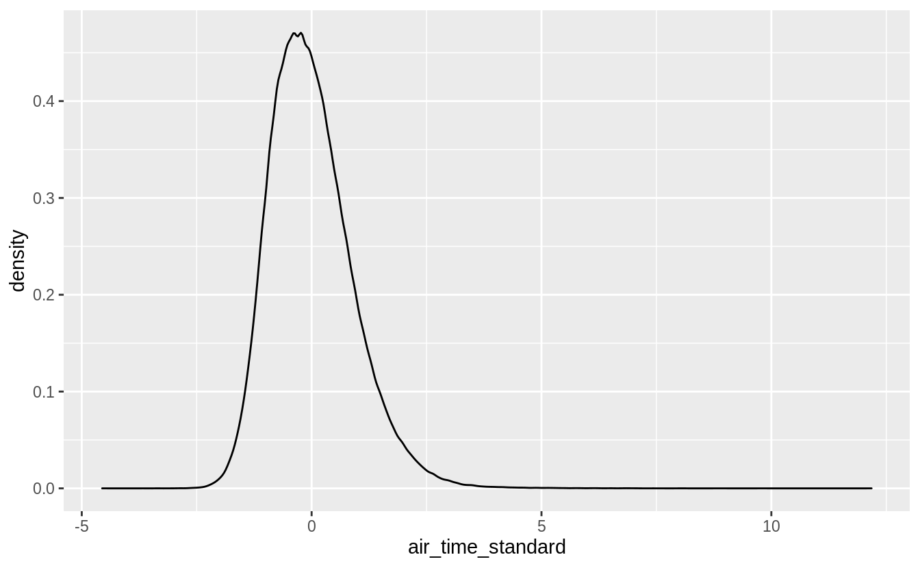
Look at each destination. Can you find flights that are suspiciously fast? (i.e. flights that represent a potential data entry error). Compute the air time of a flight relative to the shortest flight to that destination. Which flights were most delayed in the air?
使用Standardization偵測不尋常的觀察值。
standardized_flights <- flights %>%
  filter(!is.na(air_time)) %>%
  group_by(dest, origin) %>%
  #from the same origin to the same destination
  mutate(
    air_time_mean = mean(air_time),
    air_time_sd = sd(air_time),
    n = n()
  ) %>%
  ungroup() %>%
  mutate(air_time_standard = (air_time - air_time_mean) / (air_time_sd + 1))
# add 1 to the denominator and numerator to avoid dividing
# by zero
# 等價於以上程式區塊
standardized_flights <- flights %>%
  filter(!is.na(air_time)) %>%
  group_by(origin, dest) %>%
  mutate( n = n(),
         air_time_mean = mean(air_time),
         air_time_sd = sd(air_time),
         ) %>%
  mutate(standard_air_time = (air_time - air_time_mean)
         / (air_time_sd + 1 )
         ) %>%
  select(standard_air_time, everything())

ggplot(standardized_flights, aes(x = air_time_standard)) +
  geom_density()
# show the top ten outliers
standardized_flights %>%
  arrange(air_time_standard) %>%
  select(
    carrier, flight, origin, dest, month, day,
    air_time, air_time_mean, air_time_standard
  ) %>%
  head(10) %>%
  print(width = Inf) # optional to ensure that all columns will
                     # be printed ---
# use the median as a measure of central tendency and the
# interquartile range (IQR) as a measure of spread
# more robust to outliers

standardized_flights2 <- flights %>%
  filter(!is.na(air_time)) %>%
  group_by(dest, origin) %>%
  mutate(
    air_time_median = median(air_time),
    air_time_iqr = IQR(air_time),
    n = n(),
    air_time_standard = (air_time - air_time_median) / air_time_iqr
  )

ggplot(standardized_flights2, aes(x = air_time_standard)) +
  geom_density()
Knowing the substance of the data analysis at hand is one of the most important tools of a data scientist. The tools of statistics are a complement, not a substitute, for that knowledge.
Exercise 5.7.7 *****
Find all destinations that are flown by at least two carriers. Use that information to rank the carriers.
flights %>%
  # find all airports with > 1 carrier
  group_by(dest) %>%
  mutate(n_carriers = n_distinct(carrier)) %>%
  # use n_distinct() to count diff carrier
  filter(n_carriers > 1) %>%
  # rank carriers by numer of destinations
  group_by(carrier) %>%
  summarize(n_dest = n_distinct(dest)) %>%
  arrange(desc(n_dest))

Exercise 5.7.8 *******
For each plane, count the number of flights before the first delay of greater than 1 hour.
拆解問題,分為三個程式區塊實作:
#1. reconstruct the tbl
a <- flights %>%
  # sort in increasing order
  select(tailnum, year, month, day, dep_delay) %>%
  filter(!is.na(dep_delay)) %>%
  arrange(tailnum, year, month, day) %>%
  group_by(tailnum)

# 2. add a column to tbl,
# "num of flights greater than 1 hour"
b <- flights %>%
  # sort in increasing order
  select(tailnum, year, month, day, dep_delay) %>%
  filter(!is.na(dep_delay)) %>%
  arrange(tailnum, year, month, day) %>%
  group_by(tailnum) %>%
  # cumulative number of flights delayed over one hour
  # hint: use cumsum()
  mutate(cumulative_hr_delays = cumsum(dep_delay > 60))

ans <- flights %>%
  # sort in increasing order
  select(tailnum, year, month, day, dep_delay) %>%
  filter(!is.na(dep_delay)) %>%
  arrange(tailnum, year, month, day) %>%
  group_by(tailnum) %>%
  # cumulative number of flights delayed over one hour
  mutate(cumulative_hr_delays = cumsum(dep_delay > 60)) %>%
  # count the number of flights == 0
  # "count the number of flights before the first delay" ---
  summarise(total_flights = sum(cumulative_hr_delays < 1)) %>%
  arrange(total_flights)

