5.6 Grouped summaries with summarise()
summrise函數可將整個data frame濃縮成一列我們所需的資訊。
#using summarise to show "mean" of dep_delay
summarise(flights, delay = mean(dep_delay, na.rm = TRUE))

#> # A tibble: 1 x 1
#>   delay
#>   <dbl>
#> 1  12.6
summarise()搭配group_by()可以針對我們感興趣的群組列出常用統計量,相當實用。若將經過group_by()運算的 data frame 再做 summarise() , summarise() 會自動只對群組化過的資料範圍運算。( automatically applied “by group” )
by_day <- group_by(flights, year, month, day)
summarise(by_day, delay = mean(dep_delay, na.rm = TRUE))
#將會得到每日(因為已經以year,month, day 群組化資料)的平均dep_delay---
5.6.1 Combining multiple operations with the pipe
假設我們想要了解航班目的地與飛行距離、平均delay分鐘數間的關係。會使用一連串的函數運算。
by_dest <- group_by(flights, dest)
delay <- summarise(by_dest,
                   count = n(),
                   dist = mean(distance, na.rm = TRUE),
                   delay = mean(arr_delay, na.rm = TRUE)
)
# use n() to count the number of observations in the current  group---

delay <- filter(delay, count > 20, dest != "HNL")
# 只留下sample size > 20 的地點且排除dest = "HNL"的航班

# It looks like delays increase with distance up to ~750 miles
# and then decrease. Maybe as flights get longer there's more
# ability to make up delays in the air?

ggplot(data = delay, mapping = aes(x = dist, y = delay)) +
  geom_point(aes(size = count), alpha = 1/3) +
  geom_smooth(se = FALSE)
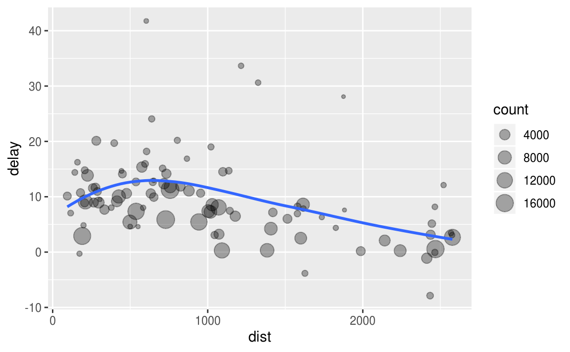
and then decrease
以上程式區塊執行了三個步驟的功能:
- Group flights by destination.
- Summarise to compute distance, average delay, and number of flights.
- Filter to remove noisy points and Honolulu airport, which is almost twice as far away as the next closest airport.
我們可以使用 pipe運算子 %>% 來簡化原本必須分段撰寫的分析。使用pipe讓我們聚焦在data frame轉換的動作上,而不用分心於中介的data frame。使用pipe同時可以增加程式碼的可閱讀性。
例如 f(x, y) 可寫作 x %>% f(y)
g(f(x, y), z) 可寫作 x %>% f(y) %>% g(z)
# group, then summarise, then filter
# a good way to pronounce %>% when reading code is “then” ---

delays <- flights %>%
  group_by(dest) %>%
  summarise(
    count = n(),
    dist = mean(distance, na.rm = TRUE),
    delay = mean(arr_delay, na.rm = TRUE)
  ) %>%
  filter(count > 20, dest != "HNL")
除了ggplot2之外,其他tidyverse中的包都可以使用pipe。
5.6.2 Missing values
若不設定 na.rm ,我們將會在data frame中看見非常多遺漏值!
flights %>%
  group_by(year, month, day) %>%
  summarise(mean = mean(dep_delay))
#> # A tibble: 365 x 4
#> # Groups:   year, month [?]
#>    year month   day  mean
#>   <int> <int> <int> <dbl>
#> 1  2013     1     1    NA
#> 2  2013     1     2    NA
#> 3  2013     1     3    NA
#> 4  2013     1     4    NA
#> 5  2013     1     5    NA
#> 6  2013     1     6    NA
#> # … with 359 more rows
因此tidyverse中所有的 aggregation function 都可以設定 na.rm 以便在計算前移除遺漏值。
flights %>%
  group_by(year, month, day) %>%
  summarise(mean = mean(dep_delay, na.rm = TRUE))
#> # A tibble: 365 x 4
#> # Groups:   year, month [?]
#>    year month   day  mean
#>   <int> <int> <int> <dbl>
#> 1  2013     1     1 11.5
#> 2  2013     1     2 13.9
#> 3  2013     1     3 11.0
#> 4  2013     1     4  8.95
#> 5  2013     1     5  5.73
#> 6  2013     1     6  7.15
#> # … with 359 more rows
# use is.na() to remove missing value from data frame

not_cancelled <- flights %>%
  filter(!is.na(dep_delay), !is.na(arr_delay))

not_cancelled %>%
  group_by(year, month, day) %>%
  summarise(mean = mean(dep_delay))
#> # A tibble: 365 x 4
#> # Groups:   year, month [?]
#>    year month   day  mean
#>   <int> <int> <int> <dbl>
#> 1  2013     1     1 11.4
#> 2  2013     1     2 13.7
#> 3  2013     1     3 10.9
#> 4  2013     1     4  8.97
#> 5  2013     1     5  5.73
#> 6  2013     1     6  7.15
#> # … with 359 more rows
5.6.3 Counts
使用 n( ) 計算觀察值(樣本個數)
sum(!is.na(x)) 計算非遺漏值的觀察值個數
# flights去除遺漏值後的data frame,將其命名為not_cancelled
not_cancelled <- flights %>%
  filter(!is.na(dep_delay), !is.na(arr_delay))

#以機型群組化後,計算平均delay分鐘數,整理為delays data frame ---
delays <- not_cancelled %>%
  group_by(tailnum) %>%
  summarise(
    delay = mean(arr_delay)
  )

# 以平均 delay 分鐘數 為 x 軸,畫出 delay 分鐘數的計次圖

ggplot(data = delays, mapping = aes(x = delay)) +
  geom_freqpoly(binwidth = 10)
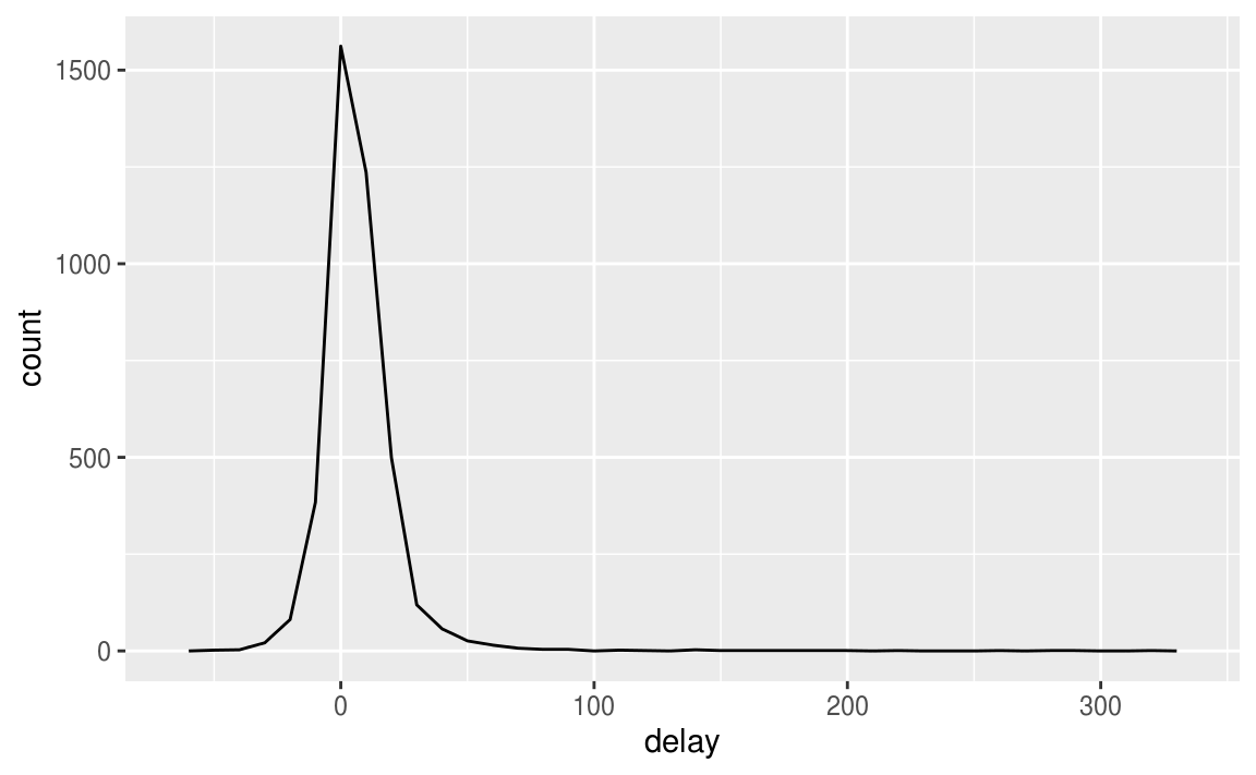
假如我們想知道平均delay分鐘數的個別次數,以下圖觀察會更清楚:
或者我們可以直接畫出各機型(tailnum)的平均delay時間:
ggplot(data = delays, mapping = aes(x = tailnum, y = delay)) +
  geom_point()

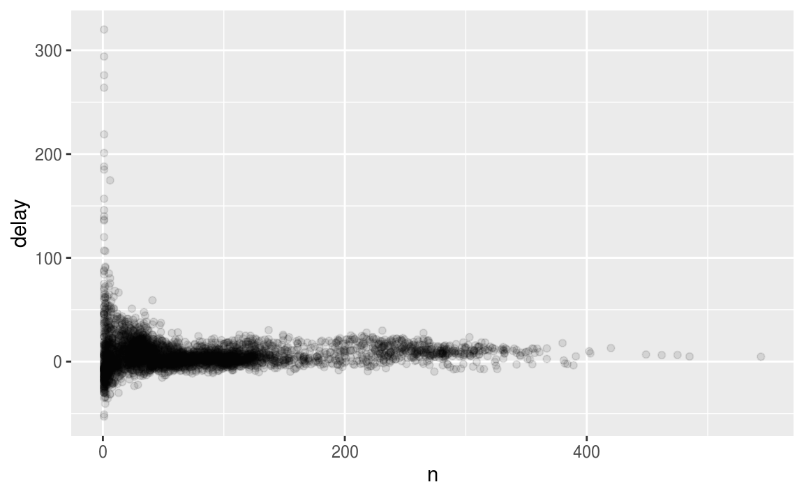
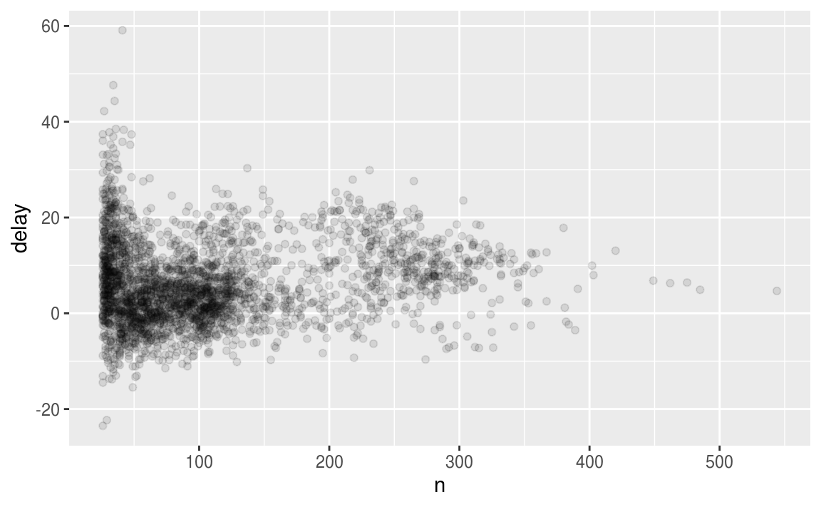
當我們忽略觀察值中樣本數太小的群組時(例如以下程式區塊:忽略樣本數小於25的機型),可以更清楚觀察到變數之間的pattern
not_cancelled <- flights %>%
  filter(!is.na(dep_delay), !is.na(arr_delay))


delays <- not_cancelled %>%
  group_by(tailnum) %>%
  summarise(
    delay = mean(arr_delay, na.rm = TRUE),
    n = n()
  )

# 注意,由於ggplot2不支援pipe,layer之間還是以 + 連接
delays %>%
  filter(n > 25) %>%
    ggplot(mapping = aes(x = n, y = delay)) +
  geom_point(alpha = 1/10)
在探索觀察值個數使用 n() 函數時,常用RStudio的快速鍵為 Cmd/Ctrl + Shift + P ,會再次傳送先前運算的程式區塊( resends the previously sent chunk from the editor to the console ),只要修改程式區塊n的個數,使用 Ctrl + Shift + P 可快速重複運行同樣的指令。
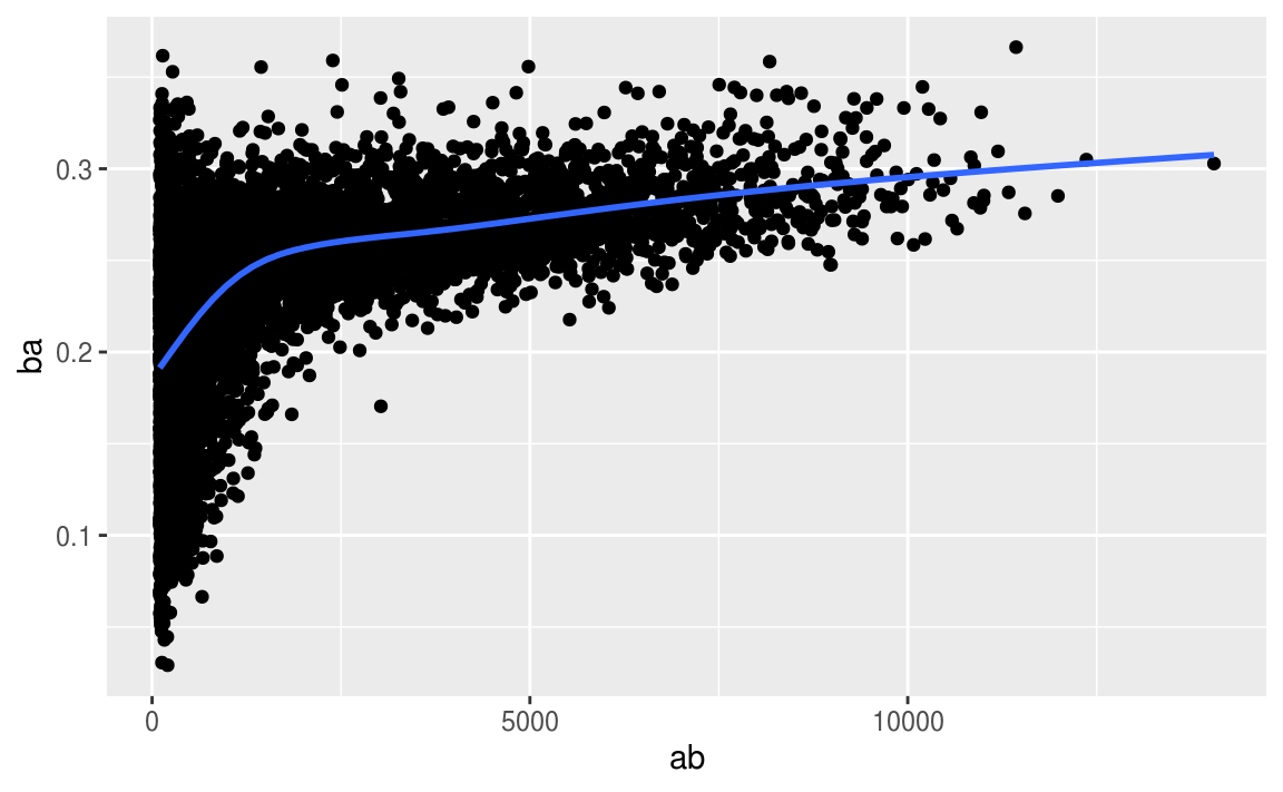
以下使用 tidyverse 中內建的 Lahman 數據集作為演練。
# Convert to a tibble so it prints nicely
batting <- as_tibble(Lahman::Batting)

batters <- batting %>%
  group_by(playerID) %>%
  summarise(
    ba = sum(H, na.rm = TRUE) / sum(AB, na.rm = TRUE),
    ab = sum(AB, na.rm = TRUE)
  )

batters %>%
  filter(ab > 100) %>%
  ggplot(mapping = aes(x = ab, y = ba)) +
    geom_point() +
    geom_smooth(se = FALSE)
#> `geom_smooth()` using method = 'gam' and formula 'y ~ s(x, bs = "cs")'
5.6.4 Useful summary functions
常見統計量的函數運算、常用指令
- 衡量中央趨勢:
mean(x),median(x) - 衡量分散趨勢:
sd(x),IQR(x),mad(x)
median absolute deviationmad(x)較不易受離群值影響。 - 衡量次序:
min(x),quantile(x, 0.25),max(x) - 衡量位置:
first(x),nth(x, 2),last(x). These work similarly tox[1],x[2], andx[length(x)]but let you set a default value if that position does not exist - 計數(Count):
n(),sum(!is.na(x)),n_distinct(x) - TRUE, FALSE 與sum( ), mean( ) 的應用:可將條件式寫進sum( ) 或 mean( ),運用函數回傳值的特性,可以輕鬆計算符合條件的觀察值個數。
When used with numeric functions,TRUEis converted to 1 andFALSEto 0. This makessum()andmean()very useful:sum(x)gives the number ofTRUEs inx, andmean(x)gives the proportion.
library(tidyverse)
library(nycflights13)

not_cancelled <- flights %>%
  filter(!is.na(dep_delay), !is.na(arr_delay))

# Measures of location
not_cancelled %>%
  group_by(year, month, day) %>%
  summarise(
    avg_delay1 = mean(arr_delay),
    avg_delay2 = mean(arr_delay[arr_delay > 0]) # the average positive delay
  )

# Measures of spread

not_cancelled %>%
  group_by(dest) %>%
  summarise(distance_sd = sd(distance)) %>%
  arrange(desc(distance_sd))

# Measures of rank
not_cancelled %>%
  group_by(year, month, day) %>%
  summarise(
    first = min(dep_time),
    last = max(dep_time)
  )

# Measures of position

not_cancelled %>%
  group_by(year, month, day) %>%
  summarise(
    first_dep = first(dep_time),
    last_dep = last(dep_time)
  )

# Measures of position within filter()

not_cancelled %>%
  group_by(year, month, day) %>%
  mutate(r = min_rank(desc(dep_time))) %>%
  filter(r %in% range(r))

# Which destinations have the most carriers?
not_cancelled %>%
  group_by(dest) %>%
  summarise(carriers = n_distinct(carrier)) %>%
  arrange(desc(carriers))

# SQLike command, count(), if all you want is a count
not_cancelled %>%
  count(dest)
#> # A tibble: 104 x 2
#>   dest      n
#>   <chr> <int>
#> 1 ABQ     254
#> 2 ACK     264
#> 3 ALB     418
#> 4 ANC       8
#> 5 ATL   16837
#> 6 AUS    2411
#> # … with 98 more rows

# count() can optionally provide a weight variable
not_cancelled %>%
  count(tailnum, wt = distance)

# 等價於 各機型 * distance
#not_cancelled %>%
#  count(tailnum, distance) ---

#> # A tibble: 4,037 x 2
#>   tailnum      n
#>   <chr>    <dbl>
#> 1 D942DN    3418
#> 2 N0EGMQ  239143
#> 3 N10156  109664
#> 4 N102UW   25722
#> 5 N103US   24619
#> 6 N104UW   24616
#> # … with 4,031 more rows

# How many flights left before 5am? (these usually indicate
# delayed flights from the previous day) ---
# Using sum( )
not_cancelled %>%
  group_by(year, month, day) %>%
  summarise(n_early = sum(dep_time < 500))

# What proportion of flights are delayed by more than an hour?
# Using mean( ) to show proportion
not_cancelled %>%
  group_by(year, month, day) %>%
  summarise(hour_perc = mean(arr_delay > 60))
5.7 Grouped mutates (and filters)
group_by( ), summarise( ) , mutate( ) , filter( ) ,以下為應用實例:
# Find the worst members of each group:

flights_sml %>%
  group_by(year, month, day) %>%
  filter(rank(desc(arr_delay)) < 10)
#> # A tibble: 3,306 x 7
#> # Groups:   year, month, day [365]
#>    year month   day dep_delay arr_delay distance air_time
#>   <int> <int> <int>     <dbl>     <dbl>    <dbl>    <dbl>
#> 1  2013     1     1       853       851      184       41
#> 2  2013     1     1       290       338     1134      213
#> 3  2013     1     1       260       263      266       46
#> 4  2013     1     1       157       174      213       60
#> 5  2013     1     1       216       222      708      121
#> 6  2013     1     1       255       250      589      115
#> # … with 3,300 more rows
# Find all groups bigger than a threshold:

popular_dests <- flights %>%
  group_by(dest) %>%
  filter(n() > 365)
popular_dests

#> # A tibble: 332,577 x 19
#> # Groups:   dest [77]
#>    year month   day dep_time sched_dep_time dep_delay arr_time
#>   <int> <int> <int>    <int>          <int>     <dbl>    <int>
#> 1  2013     1     1      517            515         2      830
#> 2  2013     1     1      533            529         4      850
#> 3  2013     1     1      542            540         2      923
#> 4  2013     1     1      544            545        -1     1004
#> 5  2013     1     1      554            600        -6      812
#> 6  2013     1     1      554            558        -4      740
#> # … with 3.326e+05 more rows, and 12 more variables: sched_arr_time <int>,
#> #   arr_delay <dbl>, carrier <chr>, flight <int>, tailnum <chr>,
#> #   origin <chr>, dest <chr>, air_time <dbl>, distance <dbl>, hour <dbl>,
#> #   minute <dbl>, time_hour <dttm>
# Standardise to compute per group metrics:

popular_dests %>%
  filter(arr_delay > 0) %>%
  mutate(prop_delay = arr_delay / sum(arr_delay)) %>%
  select(year:day, dest, arr_delay, prop_delay)
#> # A tibble: 131,106 x 6
#> # Groups:   dest [77]
#>    year month   day dest  arr_delay prop_delay
#>   <int> <int> <int> <chr>     <dbl>      <dbl>
#> 1  2013     1     1 IAH          11  0.000111
#> 2  2013     1     1 IAH          20  0.000201
#> 3  2013     1     1 MIA          33  0.000235
#> 4  2013     1     1 ORD          12  0.0000424
#> 5  2013     1     1 FLL          19  0.0000938
#> 6  2013     1     1 ORD           8  0.0000283
#> # … with 1.311e+05 more rows
