5.5 Add new variables with mutate()
mutate( ) 函數是以現有的column為基礎,在data frame中添加新column.
複習:在RStudio中,可以使用 View( ) 查看data frame的所有columns.
flights_sml <- select(flights,
                      year:day,
                      ends_with("delay"),
                      distance,
                      air_time
)
flights_sml
mutate(flights_sml,
       gain = dep_delay - arr_delay,
       speed = distance / air_time * 60
)

# You can refer to columns that you’ve just created:
mutate(flights_sml,
  gain = dep_delay - arr_delay,
  hours = air_time / 60,
  gain_per_hour = gain / hours
)
- 使用
transmute( )只列出新創的column:
transmute(flights,
  gain = dep_delay - arr_delay,
  hours = air_time / 60,
  gain_per_hour = gain / hours
)
#> # A tibble: 336,776 x 3
#>    gain hours gain_per_hour
#>   <dbl> <dbl>         <dbl>
#> 1    -9  3.78         -2.38
#> 2   -16  3.78         -4.23
#> 3   -31  2.67        -11.6
#> 4    17  3.05          5.57
#> 5    19  1.93          9.83
#> 6   -16  2.5          -6.4
#> # … with 3.368e+05 more rows
- Useful creation functions using with
mutate( )
The key property is that the function must be vectorised: it must take a vector of values as input, return a vector with the same number of values as output.
以下列出常見的用法:
- Arithmetic operators:
+,-,*,/,^.
These are all vectorised, using the so called “recycling rules”. If one parameter is shorter than the other, it will be automatically extended to be the same length. This is most useful when one of the arguments is a single number:air_time / 60,hours * 60 + minute, etc.
Arithmetic operators are also useful in conjunction with the aggregate functions(聚合函數) you’ll learn about later. For example,x / sum(x)calculates the proportion of a total, andy - mean(y)computes the difference from the mean. - Modular arithmetic:
%/%(integer division) and%%(remainder), wherex == y * (x %/% y) + (x %% y).
Modular arithmetic is a handy tool because it allows you to break integers up into pieces. For example, in the flights dataset, you can computehourandminutefromdep_timewith:
- Logs:
log(),log2(),log10(). Logarithms are an incredibly useful transformation for dealing with data that ranges across multiple orders of magnitude. They also convert multiplicative relationships to additive, a feature we’ll come back to in modelling. - Offsets:
lead()andlag()allow you to refer to leading or lagging values. This allows you to compute running differences (e.g.x - lag(x)) or find when values change (x != lag(x)). They are most useful in conjunction withgroup_by(), which you’ll learn about shortly. - Cumulative and rolling aggregates: R provides functions for running sums, products, mins and maxes:
cumsum(),cumprod(),cummin(),cummax(); and dplyr providescummean()for cumulative means. - Logical comparisons,
<,<=,>,>=,!=, and==, 邏輯運算子組合成的條件式較複雜時,建議將其條件式運算結果先存入臨時變數,確保每個步驟皆正確無誤。 - Ranking: there are a number of ranking functions, but you should start with
min_rank()是對資料進行排序,遇到重複值,排序相同,但每個值都佔一個位置,遺漏值不列入。
# An example of modular arithmetic
transmute(flights,
  dep_time,
  hour = dep_time %/% 100,
  minute = dep_time %% 100
)
#> # A tibble: 336,776 x 3
#>   dep_time  hour minute
#>      <int> <dbl>  <dbl>
#> 1      517     5     17
#> 2      533     5     33
#> 3      542     5     42
#> 4      544     5     44
#> 5      554     5     54
#> 6      554     5     54
#> # … with 3.368e+05 more rows
# lead() and lag()
# Find the "next" or "previous" values in a vector.
# Useful for comparing values ahead of or behind the # current values.
(x <- 1:10)
#>  [1]  1  2  3  4  5  6  7  8  9 10

lag(x)
#>  [1] NA  1  2  3  4  5  6  7  8  9

lead(x)
#>  [1]  2  3  4  5  6  7  8  9 10 NA
# Cumulative and rolling aggregates
x
#>  [1]  1  2  3  4  5  6  7  8  9 10

cumsum(x)
#>  [1]  1  3  6 10 15 21 28 36 45 55

cummean(x)
#>  [1] 1.0 1.5 2.0 2.5 3.0 3.5 4.0 4.5 5.0 5.5
# 常用的排序(ranking)函數
y <- c(1, 2, 2, NA, 3, 4)
min_rank(y)
#> [1]  1  2  2 NA  4  5
min_rank(desc(y))
#> [1]  5  3  3 NA  2  1

row_number(y)
#> [1]  1  2  3 NA  4  5

dense_rank(y)
#> [1]  1  2  2 NA  3  4

percent_rank(y)
#> [1] 0.00 0.25 0.25   NA 0.75 1.00

cume_dist(y)
#> [1] 0.2 0.6 0.6  NA 0.8 1.0
Exercise 5.5.1
Currently dep_time and sched_dep_time are convenient to look at, but hard to compute with because they’re not really continuous numbers. Convert them to a more convenient representation of number of minutes since midnight.
Hint: converting format HHMM to minutes since midnight(int.)
1. the integer division operator, %/%
2. the modulo operator, %%
3. now, we can convert all the times to minutes after midnight
4. x %% 1440 will convert 1440 to zero while keeping all the other times the same, this step will convert midnight(24:00 equals 1440 mins) to zero.
# convert HHMM to minutes after midnight
# convert 24:00 to zero
flights_times <- mutate(flights,
  dep_time_mins = (dep_time %/% 100 * 60 + dep_time %% 100) %% 1440,
  sched_dep_time_mins = (sched_dep_time %/% 100 * 60 +
    sched_dep_time %% 100) %% 1440
)

# view only relevant columns
select(
  flights_times, dep_time, dep_time_mins, sched_dep_time,
  sched_dep_time_mins
)
#> # A tibble: 336,776 x 4
#>   dep_time dep_time_mins sched_dep_time sched_dep_time_mins
#>      <int>         <dbl>          <int>               <dbl>
#> 1      517           317            515                 315
#> 2      533           333            529                 329
#> 3      542           342            540                 340
#> 4      544           344            545                 345
#> 5      554           354            600                 360
#> 6      554           354            558                 358
#> # … with 3.368e+05 more rows
# define a function to avoid copying and pasting code
time2mins <- function(x) {
  (x %/% 100 * 60 + x %% 100) %% 1440
}


#Using time2mins, the previous code simplifies to the following.


flights_times <- mutate(flights,
  dep_time_mins = time2mins(dep_time),
  sched_dep_time_mins = time2mins(sched_dep_time)
)
# show only the relevant columns
select(
  flights_times, dep_time, dep_time_mins, sched_dep_time,
  sched_dep_time_mins
)
#> # A tibble: 336,776 x 4
#>   dep_time dep_time_mins sched_dep_time sched_dep_time_mins
#>      <int>         <dbl>          <int>               <dbl>
#> 1      517           317            515                 315
#> 2      533           333            529                 329
#> 3      542           342            540                 340
#> 4      544           344            545                 345
#> 5      554           354            600                 360
#> 6      554           354            558                 358
#> # … with 3.368e+05 more rows
Exercise 5.5.2
Compare air_time with arr_time - dep_time. What do you expect to see? What do you see? What do you need to do to fix it?
# define air-time = arr_time - dep_time
flights_airtime <-
  mutate(flights,
    dep_time = (dep_time %/% 100 * 60 + dep_time %% 100) %% 1440,
    arr_time = (arr_time %/% 100 * 60 + arr_time %% 100) %% 1440,
    air_time_diff = air_time - arr_time + dep_time
  )

# If air_time = arr_time - dep_time , there should be no flights with non-zero values of air_time_diff.
# use nrow to calculate numbers of rows
nrow(filter(flights_airtime, air_time_diff != 0))
#> [1] 327150
除了數據錯誤之外,可能有下列的原因造成airtime != arr_time – dep_time
- 抵達時間為清晨,所以arr_time 數值小於 dep_time。若屬於此種狀況,
airtime 將小於24:00(即1440分鐘) - 飛行跨越時區,airtime被時差抵銷,data set為啟程自紐約市的國內航班,因此時區造成的時間差(即airtime 與 arr_time – dep_time的差距)會是60的倍數(60 minutes (Central) 120 minutes (Mountain), 180 minutes (Pacific), 240 minutes (Alaska), or 300 minutes (Hawaii))
不論是以上哪種情況,時間差應該皆是60的倍數。對此針對時間差作圖,求證假設。
ggplot(flights_airtime, aes(x = air_time_diff)) +
  geom_histogram(binwidth = 1)
#> Warning: Removed 9430 rows containing non-finite values (stat_bin).
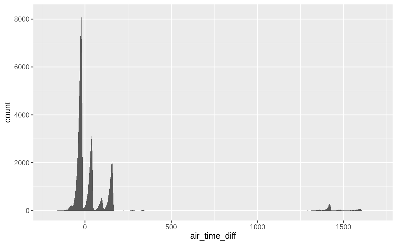
由上圖可知大多數的時間差並非是60的倍數,即上述假設不成立。進一步我們過濾出目的地為洛杉磯的班機,其時間差應該是180分鐘。並作圖驗證之。
ggplot(filter(flights_airtime, dest == "LAX"), aes(x = air_time_diff)) +
  geom_histogram(binwidth = 1)
#> Warning: Removed 148 rows containing non-finite values (stat_bin).
重新觀察documentation,發現時間差可能由於未考慮牽引機拖班機進Bay的時間,所以欄位間關係不如預期。顯示核對column定義的重要性。
Exercise 5.5.3
比較 dep_time, sched_dep_time, dep_delay 這些column之間,應該會有 dep_time – sched_dep_time = dep_delay的關係。
flights_deptime <-
  mutate(flights,
    dep_time_min = (dep_time %/% 100 * 60 + dep_time %% 100) %% 1440,
    sched_dep_time_min = (sched_dep_time %/% 100 * 60 +
      sched_dep_time %% 100) %% 1440,    #先將時間格式轉換為分鐘 ---
    dep_delay_diff = dep_delay - dep_time_min + sched_dep_time_min
  # 添加一個新欄位 dep_delay_diff 定義如上行code ---
  )
# 由我們的定義可知 dep_delay_diff 中每一 row 的數值應該為 0
# 驗證之---

filter(flights_deptime, dep_delay_diff != 0)
#> # A tibble: 1,236 x 22
#>    year month   day dep_time sched_dep_time dep_delay arr_time
#>   <int> <int> <int>    <int>          <int>     <dbl>    <int>
#> 1  2013     1     1      848           1835       853     1001
#> 2  2013     1     2       42           2359        43      518
#> 3  2013     1     2      126           2250       156      233
#> 4  2013     1     3       32           2359        33      504
#> 5  2013     1     3       50           2145       185      203
#> 6  2013     1     3      235           2359       156      700
#> # … with 1,230 more rows, and 15 more variables: sched_arr_time <int>,
#> #   arr_delay <dbl>, carrier <chr>, flight <int>, tailnum <chr>,
#> #   origin <chr>, dest <chr>, air_time <dbl>, distance <dbl>, hour <dbl>,
#> #   minute <dbl>, time_hour <dttm>, dep_time_min <dbl>,
#> #   sched_dep_time_min <dbl>, dep_delay_diff <dbl>
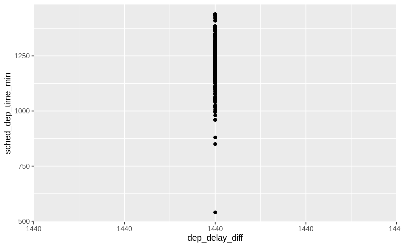
結果有1236 rows不為零,可能的原因是班機於24:00前起飛,但在24:00後(midnight)逾時落地,若屬於此種狀況,dep_delay_diff 應該為1440,繪圖驗證之:
ggplot(
  filter(flights_deptime, dep_delay_diff > 0),
  aes(y = sched_dep_time_min, x = dep_delay_diff)
) +
  geom_point()
Find the 10 most delayed flights using a ranking function. How do you want to handle ties? Carefully read the documentation for min_rank()
dplyr包有許多用來排序的函數: row_number(), min_rank(), dense_rank() ,對於重複值(ties)各有不同的處理方式。以下內容摘錄自 https://www.cnblogs.com/wkslearner/p/5768845.html
min_rank()是对数据大小进行编号排序,遇到重复值,排序相同,但每个值都占一个位置,缺失值不计入 。
row_number()是对数据大小进行编号排序,遇到重复值,排序继续加1,缺失值不计入 。
其運算結果與index(or row number) of each element相同。
dense_rank() 是对数据大小进行编号排序,遇到重复值,排序相同,所有重复值只占一个位置,缺失值不计入 。
對於ties的處理與min_rank相同,但是對於tie的next rank有不同處理。如以下程式碼:
# create a seq, naming temp
(temp <- c(8, 1, 8, 2, 9, 5, 2, 8) )
#> [1] 8 1 8 2 9 5 2 8

(min_rank(temp))
#> [1] 5 1 5 2 8 4 2 5
# 重複值的每個元素都占用一個位置

(dense_rank(temp))
#> [1] 4 1 4 2 5 3 2 4
# 遇到重複值,所有重複值只佔一個位置
以下範例可看出這些ranking function的不同之處。
# create a tibble, which naming rankme
rankme <- tibble(
  x = c(10, 5, 1, 5, 5)
)

# using mutate() to add column
rankme <- mutate(rankme,
                 x_row_number = row_number(x),
                 x_min_rank = min_rank(x),
                 x_dense_rank = dense_rank(x)
)

# show the difference between ranking functions
# using arrange(dataframe, var.to reorder column)
arrange(rankme, x)
若沒有特別指定,通常使用min_rank()函數排序。
以下程式碼可以列出前十delayed_flights。
flights_delayed <- mutate(flights,
  dep_delay_min_rank = min_rank(desc(dep_delay)),
  dep_delay_row_number = row_number(desc(dep_delay)),
  dep_delay_dense_rank = dense_rank(desc(dep_delay))
)

#只留下前十遲到班機,top_n()要配合 >%>運算子,容後再述---
flights_delayed <- filter(
  flights_delayed,
  !(dep_delay_min_rank > 10 | dep_delay_row_number > 10 |
    dep_delay_dense_rank > 10)
)

#reorder by dep_delay_min_rank
flights_delayed <- arrange(flights_delayed, dep_delay_min_rank)

print(select(
  flights_delayed, month, day, carrier, flight, dep_delay,
  dep_delay_min_rank, dep_delay_row_number, dep_delay_dense_rank
),
n = Inf
)
#> # A tibble: 10 x 8
#>    month   day carrier flight dep_delay dep_delay_min_r… dep_delay_row_n…
#>    <int> <int> <chr>    <int>     <dbl>            <int>            <int>
#>  1     1     9 HA          51      1301                1                1
#>  2     6    15 MQ        3535      1137                2                2
#>  3     1    10 MQ        3695      1126                3                3
#>  4     9    20 AA         177      1014                4                4
#>  5     7    22 MQ        3075      1005                5                5
#>  6     4    10 DL        2391       960                6                6
#>  7     3    17 DL        2119       911                7                7
#>  8     6    27 DL        2007       899                8                8
#>  9     7    22 DL        2047       898                9                9
#> 10    12     5 AA         172       896               10               10
#> # … with 1 more variable: dep_delay_dense_rank <int>
Exercise 5.5.5
What does 1:3 + 1:10 return? Why?
在R語言中基本的資料運算單位是向量(vector), 任何運算都是元素級別(element-wise)和函數以映射方式應用到每個元素之上 。
1:3 + 1:10
#> Warning in 1:3 + 1:10: longer object length is not a multiple of shorter
#> object length
#>  [1]  2  4  6  5  7  9  8 10 12 11
# 1:3 + 1:10 等於
c(1 + 1, 2 + 2, 3 + 3, 1 + 4, 2 + 5, 3 + 6, 1 + 7, 2 + 8, 3 + 9,
1 + 10)

#>  [1]  2  4  6  5  7  9  8 10 12 11

a <- 1:12
b <- 1:3
a + b
[1]  2  4  6  5  7  9  8 10 12 11 13 15

# 1:3 + 1:12 等於
c(1 + 1, 2 + 2, 3 + 3, 1 + 4, 2 + 5, 3 + 6, 1 + 7, 2 + 8, 3 + 9,
1 + 10, 2 + 11, 3 + 12)
# mapping element-wise vector 1:3 four cycles to 1:12
Exercise 5.5.6
R 語言中提供的三角函數類運算函數,可使用?Trig 開啟help page.
